A Brief Introduction to Explainable AI (XAI)
October 12, 2024
Deep learning, a powerful tool in computer vision, security, and healthcare, has revolutionized how machines make decisions. However, there's a catch—these models appear as black-boxes to us. They make predictions, but it's hard for us to grasp how. This is because deep learning models learn a complex non-linear mapping between the data and the target label, parameterized by millions of weights, making it impossible to understand how a model makes a certain prediction on test cases. In many cases, such models are proprietary; hence, access to how the models were designed is limited. This opaque nature poses challenges in assessing their fairness, bias, and reliability. Imagine relying on a system for critical decisions without knowing how it works—risky, right?
The Need for XAI
That's where eXplainable Artificial Intelligence (XAI) steps in. XAI aims to demystify the decision-making process of these sophisticated models. There are two main avenues in XAI research: interpretable machine learning and explainability.
Interpretable Machine Learning: Designing Decipherable Models
The Challenge: Creating models that are naturally easy to understand.
Imagine models that, by their very design, are interpretable. Linear regression, decision trees, and generalized additive models fall into this category. With such models, you can clearly see the relationship between input features and the output label and understand how a model makes decisions for test cases. However, achieving high performance with interpretable models, especially with raw data like images, text, and videos, is not easy.
There is a growing concern in the deep learning community that reliance on explainability alone is not sufficient, and the best way to move forward is to design inherently interpretable models, even for datasets like images.
Unveiling the Black Box: Explainability Methods
The Game Plan: Unveiling how a model makes decisions.
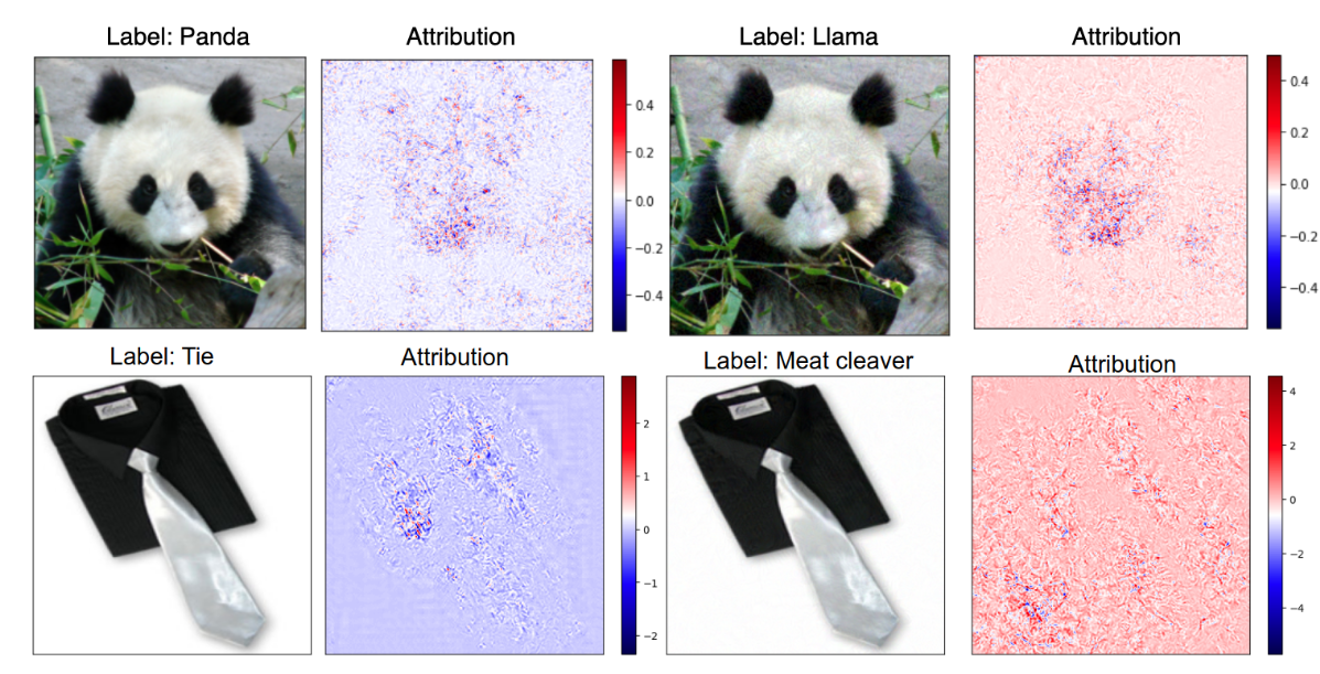
Explainability methods aim to inspect a model's predictions after it's been trained (post-hoc methods). These methods help us understand why a machine learning model made a specific decision on a given instance. One popular approach in computer vision is the use of heatmaps to visualize where a model focuses on an image during prediction.
XAI methods can be classified based on different factors:
- Local vs. Global: Does the method explain model prediction on a single instance (local) or explain the overall behavior of the model on a dataset (global)?
- Model-Agnostic vs. Model-Specific: Does the method work for any model, or is it designed for a specific architecture?
- Types of Explanation: Feature attribution, concepts, rules, or counterfactual examples.
Feature Attribution Methods
What's the Deal? Understanding the impact of individual features on predictions.
Given a trained model \( f(.) \) and a test instance \( x \in R^d \), a feature attribution-based explanation method \( \phi(x) \) returns a vector \( \phi(x) \in R^d \) that provides the importance vector of the feature.
LIME: Shining a Light Locally
High-level idea: Generate local explanations by perturbing inputs.
LIME creates an interpretable surrogate model through linear regression. Given a test instance it wants to explain, it perturbs the sample and generates new data samples to train the surrogate model. It assigns a specific weight to the sample based on its proximity to the original data point. Once you train a surrogate model, a linear regression, the weights of this model explain the predictions, with higher positive weights indicating the features that contribute the most.
Pitfalls: LIME's assumptions on feature independence might lead to unreliable insights. Their explanations are also susceptible to manipulation. LIME is also generally suitable for tabular data and not prefered for raw datasets like images and text.
SHAP: Playing the Fairness Game
High-level idea: Distributing 'credit' fairly among features.
Picture your model as a team. SHAP values use game theory to ensure each player (feature) gets a fair share of the victory. It considers all possible feature combinations and calculate the average contribution of each feature to the model's output. Like LIME, SHAP generates new samples around a given instance, obtains predictions from the black box model, and trains an interpretable linear model on the dataset. However, unlike LIME, SHAP assigns weights to the new instances based on the weight a coalition would receive in the Shapley value estimation rather than their proximity to the original sample.
Pitfalls: SHAP is computationally expensive but provides consistent results across different runs.
Gradient-Based Methods
Gradient methods compute how much the output predictions change when the input features change using the input-gradient (the gradient of model output with respect to input).
Vanilla Gradient, computes the gradient of the class score with respect to the input. This gradient quantifies how much the output predictions change when the input features change. This score serves as a measure of feature attribution. A simple enhancement to this method, called GradientXInput, involves multiplying the gradient by the input features. Vanilla gradient method computes the gradient of the output with respect to the input feature, and in some cases, even if a neural network heavily relies on a particular feature, the gradient of the class score related to that feature may have small magnitudes. This issue can arise in deep neural networks (DNNs) due to saturation during the training process. To address this challenge, the integrated gradient (IG) method accumulates gradients along a linear path from a chosen baseline to the given test sample rather than relying on simple gradients. The selection of the baseline depends on the specific application, but usually a zero baseline vector is considered. SmoothGrad and NoiseGrad propose improvements over gradient-based explanation methods. In SmoothGrad, for a given test sample, Gaussian noise is added to generate multiple samples, and their feature attributions are averaged to calculate the final attribution. On the other hand, NoiseGrad introduces noise to the model parameters, generates "n" models, and obtains an ensemble of explanations. GradientSHAP combines concepts from SHAP, SmoothGrad, and integrated gradient. Instead of selecting a single baseline, it randomly picks a baseline from a distribution of baselines, often sourced from the training set. It computes attributions for each of these baselines and then averages the results. How do you select the baseline in IG? How do you find the best noise parameter in NoiseGrad and SmoothGrad? Gradient-based explanation methods can also assist attackers in better-estimating gradients for black-box attacks and may even enable them to reconstruct the underlying model. Worrisome, right?Reality check
Feature attribution based methods are not perfect. Many methods show class-invariant behavior (they produce similar feature attributions regardless of the predicted class). They are susceptible to adversarial manipulations. An adversary (attacker) can change the attribution without changing the model prediction. Additionally, some of these methods have been found to be non-robust to changes in model parameters. Even when random numbers are used to replace the parameters of a trained neural network, the feature attributions remain relatively unchanged. In addition, explanation methods can also exhibit instability in their results, questioning their reliabilility.
Concept-Based Explanations
What's the Twist? Moving beyond pixel-level features to high-level human concepts.
Why?Pixels might not mean much to us, but shapes, patterns, and objects do. Concept-based explanation methods bridge this gap.
For example: if you have a doctor vs nurse classifier and want to inspect if the model is biased towards the gender Male in making doctor classification, how can you check that using feature attribution method? Think about it for a while.
You cannot. Feature attribution-based methods explain model prediction in terms of input features, which are pixels in images. However, such features are not user-friendly. In images, a single pixel does not represent meaningful information as we are more concerned with a group of pixels in the form of shapes, objects, colors or patterns. Concept-based explanation methods were proposed to handle such limitations. This is a fairly new research topic with some progress in recent years.
A concept in a concept-based explanation is an abstraction for high-level features interpretable to humans, like colors, shapes, patterns, and objects. The goal of a concept-based method is to inspect whether the deep learning model used such high-level human ideas in making its classification decision.
Some recent works
TCAV paper proposed a supervised approach to inspect whether a model used a concept for prediction and how important was it. To do so, it computes a vector called Concept Activation Vector (CAV), which is a representation of the defined concept in the activation space of a trained model. To compute this vector for an image classifier, we first collect a dataset of images that represents the defined concept and a dataset of random counterexamples. For example: to obtain a vector for a concept called eyes, we collect lots of images of eyes and a set of random counter examples like images of nose, hair, shoes, etc. We pass these images to the neural network and collect activations from a hidden layer of the trained network. Then, we train a binary classifier that separates the activations vectors of concept-dataset and counter-examples. The concept activation vector is a vector orthogonal to this binary classifier. Once we have the concept vector, we can measure its importance or conceptual sensitivity on a given input by computing the derivative of the model prediction on the given input in the direction of the CAV.
There are a few limitations to this method: TCAV performs badly on shallower neural networks since a shallow network might not generate activations that are linearly separable. TCAV also requires human annotation of datasets, which can be error-prone and an expensive task.
ACE, Automated Concept-based Explanation (ACE), proposes an automated process to collect CAVs using segmentation and clustering. However, such segmentation and clustering-based approaches might lose important concepts in the image. ICE avoids this clustering step and modifies the ACE framework using matrix factorization for feature maps. While ACE only provides global explanations for classes, ICE can provide local and global explanations. Since ICE takes information from only one layer, the last layer and concepts are formed gradually along the multiple hidden layers; this approach also loses some important information. We also have to predefine the number of concept components we want to obtain from a class of images. CRAFT also uses matrix factorization to identify concepts. However, in addition to extraction of concepts, it also propagates them to input features and visualizes saliency maps. Few methods have been proposed using generative networks like VAE and GANs to learn concepts from the latent representation of a neural network.
There are few problems with concept-based explanation approach: how do we verify the correctness of the discovered concepts? What if the neural network uses different reasoning for prediction instead of human-understandable concepts? How can these methods be applicable to text or tabular data?
Wrapping It Up
Explainable AI is crucial for trusting and understanding the decisions made by complex models. Feature attribution and concept-based methods are some of the tools, each with its strengths and limitations. Understanding them and improving them brings us one step closer to reliable and trustworthy AI.