Understanding Attention and Transformer
October 12, 2024
Vanilla RNNs encode word embedding in linear fashion following the principle that nearby words affect the meaning of a sentence. So, the number of steps required for distant word pair interaction grows linearly in \( O(sequence\_length) |). This introduces difficulty in learning long distance dependencies because of vanishing gradient problem over long sequence. Encoder of a vanilla RNN uses only one hidden state to capture all information of the input sequence. This causes an information bottleneck. We should extract as much information as possible from our input sequence for decoder part.
For example: in given picture, we want to translate an input sentence in English to Nepali target sentence "ma keta ho". For this type of translation task, one uses a sequence-to-sequence model, which consists of an encoder and a decoder, both of which are RNNs. In encoder, each word produces a hidden vector (called context vector) and output vector. The context vector is passed onto the next word (time). The final hidden state (context vector) is passed onto the decoder part, to translate the sentence.

To improve long-distance dependencies by solving bottleneck and vanishing gradient problems, attention was proposed. It is a mechanism by which at each time step of decoder, we use direct connection with encoder that allows us to focus on a particular part of the sentence. By connection, it means that instead of just passing one context vector, all hidden states are passed to the decoder. Attention also provides some interpretability by learning where a decoder is focusing on. Another issue with recurrent models is lack of parallelizability that inhibits training on very large dataset. Attention eases parallelization. Transformer, the most popular NLP architecture, uses attention mechanism.
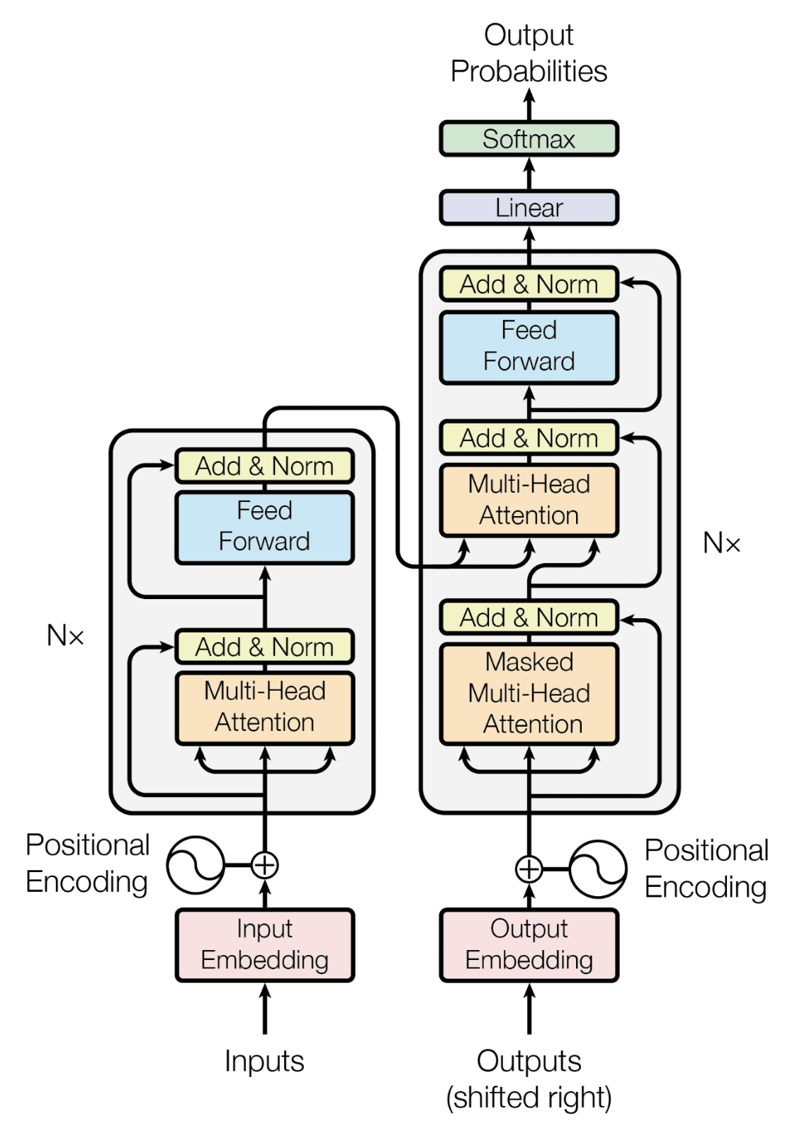
Now, lets talk about the transformer model and break it down. At the core of the Transformer model is the self-attention mechanism (which we briefly discussed just now but we will get back to it). This mechanism allows the model to weigh the importance of different words in a sequence.Input Embeddings and Tokenization
As shown in the Transformer architecture, a Transformer model starts with input embeddings, which convert words or subwords into numerical representations. Since neural networks operate on numbers, text input must be tokenized and mapped to fixed-size vectors. Tokenization tokenizes or breaks the sentence into words, subwords, or characters. Then, every token is assigned a unique numerical ID based on a fixed vocabulary. Each token ID is then mapped to a high-dimensional dense vector using a learned embedding matrix. Mathematically, if a vocabulary has \(V\) tokens and the embedding dimension is \(d_model\), then the embedding matrix \(E\) is of shape \(V, d_model\). Given a token \(t_i\) with index \(i\) in the vocabulary, its embedding is retrieved as: \[ \mathbf{e}_i = E[i] \] Initially, the embedding matrix is randomly initialized (e.g., using Gaussian initialization) and is learned through training via backpropagation. Since embeddings capture semantic meaning, words with similar meanings tend to have similar vector representations.Positional Encodings
Unlike RNNs, Transformers do not have inherent sequential processing. To incorporate word order, positional encodings are added to embeddings. These encodings help the model recognize which words appear earlier or later in a sequence. But positional encodings are not learned but instead computed once using sine and cosine functions. These functions provide a continuous pattern that allows the model to generalize to different sequence lengths. For a position \(pos\) and embedding dimension \(d_model\), the encoding is computed as: \[ PE_{(pos, 2i)} = \sin\left(\frac{pos}{10000^{2i/d_{model}}}\right) \] \[ PE_{(pos, 2i+1)} = \cos\left(\frac{pos}{10000^{2i/d_{model}}}\right) \] where \(i\) is the index of a dimension in the embedding vector. Since sine and cosine functions form a periodic pattern, they help the model recognize relative positions effectively. The positional encoding is added element-wise to the input embeddings before being passed into the encoder: \[ \mathbf{x}_i = \mathbf{e}_i + PE_i \]Self-Attention Mechanism
The self-attention mechanism enables the model to relate different words in a sentence. Instead of processing tokens sequentially, self-attention computes dependencies between all words at once. This is done using three vectos created from the input token: Query, Key, and Value. In transformer encoder, these are multiplied with learned weight matrices, and final Q,K,V computed as: \[ Q = X W_Q, \quad K = X W_K, \quad V = X W_V \] where, \(W_Q, W_K\), and \(W_V\) are learnable weight matrices. The attention score between two words is computed using the dot product of their query and key vectors: \[ \text{score} = Q K^T \] To prevent excessively large values, the score is scaled by the square root of the embedding dimension \(d_k\): \[ \text{Attention}(Q, K, V) = \text{softmax} \left( \frac{QK^T}{\sqrt{d_k}} \right) V \] The softmax function ensures that attention scores sum to 1, making them interpretable as probabilities. This attention mechanism allows words to influence each other dynamically, depending on their learned relationships. To prevent words from attending to future words during training, a masking mechanism sets certain values to `-∞` before applying softmax. This ensures that a word only considers past words during decoding.Multi-Head Attention
Transformer however uses multihead attentions which means instead of using a single attention mechanism, it uses multiple parallel attention heads. Each head focuses on different relationships between words. For each head \(i\), separate weight matrices are used. \[ \text{head}_i = \text{Attention}(QW_Q^i, KW_K^i, VW_V^i) \] The outputs of all heads are concatenated and projected using another matrix \(W_O\): \[ \text{MultiHead}(Q, K, V) = \text{Concat}(\text{head}_1, ..., \text{head}_h) W^O \] This allows the model to capture multiple types of relationships in parallel. The following figure from Umar Jamil should make things more clear on how multi-head attention is computed.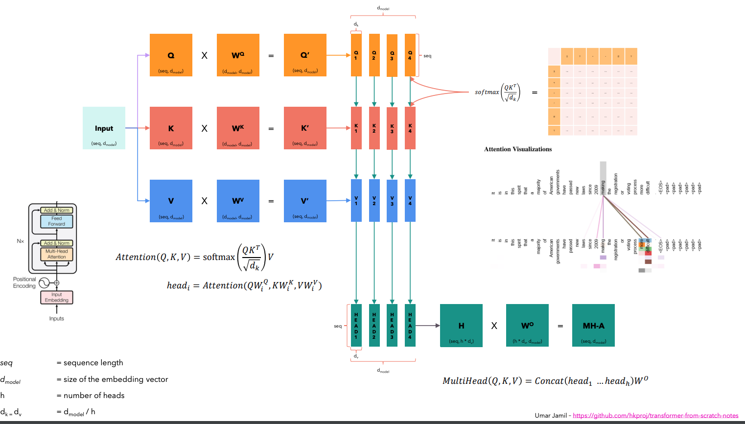 After multi-head attention, the output is added back to the original input embedding (residual connection) and normalized using layer normalization:
\[
\text{Norm}(\mathbf{x}) = \frac{\mathbf{x} - \mu}{\sigma}
\]
where \(μ\) and \(σ\) are the mean and standard deviation of the input. This helps stabilize training and prevents vanishing/exploding gradients. Now, this becomes the output of the encoder block,
which becomes Key and Value for the decoder side.
After multi-head attention, the output is added back to the original input embedding (residual connection) and normalized using layer normalization:
\[
\text{Norm}(\mathbf{x}) = \frac{\mathbf{x} - \mu}{\sigma}
\]
where \(μ\) and \(σ\) are the mean and standard deviation of the input. This helps stabilize training and prevents vanishing/exploding gradients. Now, this becomes the output of the encoder block,
which becomes Key and Value for the decoder side.
Decoder
In the decoder side, Query comes form the output embeddings (eg, target sentence). The input embedding and positional encoding is computed same as the encoder side. The decoder then follows a similar structure as the encoder but with different attention mechanism: masked multi-head attention. This satisfies our goal of making the model causal: the output at a certain position can only depend on the words on the previous positions. The model must not be able to see future words. We can do this by replacing all the values above the diagonal with \(\infty\) before applying the softmax. The final fully connected layer generates the predicted token probabilities.References
[Vaswani et al. 2017] Attention Is All You Need
[The Illustrated Transformer] https://jalammar.github.io/illustrated-transformer/
[Transformer from scratch] https://github.com/hkproj/transformer-from-scratch-notes/blob/main/Diagrams_V2.pdf