Understanding Attention and Transformer
October 12, 2024
Matrix factorization is a powerful technique used in various fields such as machine learning, data analysis, and recommender systems. At its core, matrix factorization involves decomposing a matrix into multiple matrices, typically of lower rank, to extract meaningful patterns and latent features. By representing the original matrix in terms of its constituent parts, matrix factorization enables dimensionality reduction, noise reduction, and capturing underlying structure within the data.
What is NMF?
Non-negative Matrix Factorization (NMF) is a specialized form of matrix factorization that imposes additional constraints on the decomposition process. Unlike traditional matrix factorization methods, NMF requires that all elements in the original matrix and the resulting factor matrices be non-negative. This constraint makes NMF particularly useful for data that naturally occurs in non-negative spaces, such as images, text documents, and audio signals.
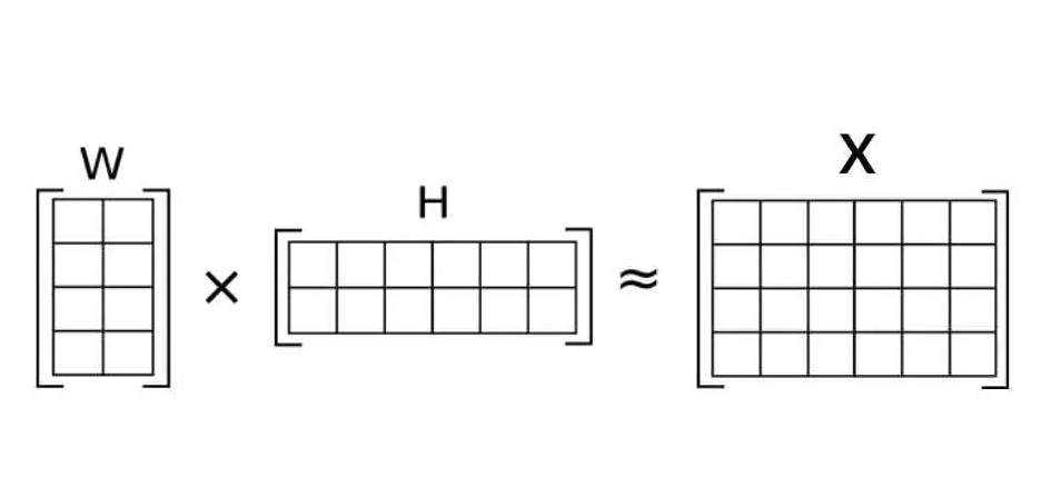
In NMF, the original matrix \(X\) is factorized into two matrices, \(W\) and \(H\), such that
\[ X \approx WH \]Where:
- \(X \in R^{M\times N}_+\)
- \(W \in R^{M\times r}_+\)
- \(H \in R^{r \times N}_+\)
The parameter \(r\) is called the approximation rank. The key characteristic of NMF is that all elements of \(W\) and \(H\) are constrained to be non-negative, which allows for an intuitive interpretation of the resulting factors as additive parts.
What does this approximation signify?
The above equation for NMF can be rewritten column-wise as \(x \approx Wh\), where \(x\) and \(h\) are corresponding columns of the matrix \(X\) and \(H\). This indicates that, with this factorization, we are approximating the data vector \(x\) by a linear combination of the columns in \(W\) weighted by the components in \(h\). This means that the matrix \(W\) contains new basis vectors optimized for the linear approximation of the original data in \(X\). A good approximation can be achieved if the basis vectors can discover the underlying structure from the data.
Solving the Optimization
To solve this optimization, we need to define a cost function that we can minimize using optimization techniques like gradient descent. One of the most common cost functions is the Frobenius norm, where the distance between the original data vector and the approximation is computed as:
\[ D(X \mid WH) = \| X - WH \|^2_F \]where,
\[ \| A - B\|^2_F = \sum_{ij} (A_{ij} - B_{ij})^2 \]Our optimization problem for NMF can be defined as:
\[ W^*, H^* = \arg\min_{W\geq 0,H \geq 0} \frac{1}{2} \| X - WH \|^2_F \]We cannot minimize this cost function jointly with respect to both \(W\) and \(H\), hence, an alternating technique is used. Minimization is performed for each variable separately at each iteration, keeping the other one fixed.
Gradient Computation
We first compute the gradient with respect to \(W\) while keeping \(H\) fixed:
\[ \nabla_W \frac{1}{2} \| X - WH \|^2_F = - X H^T + W H H^T \]The update rule for \(W\) is given by:
\[ W_{ij} \leftarrow W_{ij} + \eta_{ij} (X H^T - W H H^T)_{ij} \]The multiplicative update rule by Lee and Seung uses:
\[ \eta_{ij} = \frac{W_{ij}}{(W H H^T)_{ij}} \]This modifies the update rule to:
\[ W_{ij} \leftarrow W_{ij} \frac{(X H^T)_{ij}}{(W H H^T)_{ij}} \]Similarly, for \(H\), keeping \(W\) fixed:
\[ \nabla_H \frac{1}{2} \| X - WH \|^2_F = -W^T X + W^T W H \]and the update rule is:
\[ H_{ij} \leftarrow H_{ij} \frac{(W^T X)_{ij}}{(W^T W H)_{ij}} \]Is NMF better than other factorization methods?
NMF is often preferred if the original data matrix has non-negative values for the following reasons:
- Parts-Based Representation: NMF provides a parts-based representation of data, which is useful in image processing and text mining.
- Interpretability: The non-negativity constraint leads to more interpretable factors.
- Dimensionality Reduction: NMF reduces computational complexity and overfitting in high-dimensional datasets.
- Sparsity: NMF tends to produce sparse representations, aiding efficient computation.
However, NMF has challenges, such as being NP-hard, requiring alternating optimization, and being ill-posed due to multiple equivalent factorizations. Regularization techniques, such as sparsity constraints, help mitigate these issues.